Part 2 of 3 in the Java Performance Optimization series. ← Part 1 · Part 3 coming soon.
In Part 1 I listed eight Java performance anti-patterns and explained what each one costs at the JVM level. I also opened with some numbers I didn’t fully explain: 1,198ms down to 239ms, over 1GB of heap down to 139MB, 19 GC pauses down to 4.
This post is where those numbers come from.
We’re going to open the Java Flight Recording (JFR) from my demo app in JDK Mission Control (JMC) and actually look at what’s hot. The thing I want to show isn’t just before and after. It’s what happens in between. Fix the biggest problem and something that was invisible before suddenly shows up. The shape of the profile changes. You end up doing this in rounds, not in one pass.
The App
The demo app is an order analytics pipeline. It generates synthetic orders, validates them, computes revenue by currency, scores each order for fraud risk, detects hourly volume trends, and accumulates the results into a summary report. Nothing too crazy. I wrote it intentionally with several of the anti-patterns from Part 1 sprinkled in, to reflect what might happen in a real production system. These types of anti-patterns can naturally accumulate in a real codebase over time.
The load test processed 100,000 orders in batches of 1,000 across 100 virtual threads and collected the JFR recording.
Opening the Recording
If you haven’t used JMC before, here’s how you can do it. You can generate a .jfr file from your running process using the JDK’s built-in profile settings:
java -XX:StartFlightRecording=filename=recording.jfr,settings=profile -jar myapp.jarOr attach to a running process:
jcmd <pid> JFR.start duration=120s filename=recording.jfr settings=profileThen open it in JMC. It’s free and open source. The settings=profile part matters because it enables a broader set of events including allocation tracking, GC details, and thread contention, which you’ll want.
The first screen you land on is the Java Application overview. CPU usage, heap usage, GC activity, thread count, all plotted over the recording window. Before I changed anything, it looked like this:
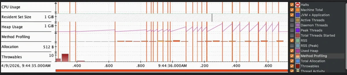
The heap pattern is the first thing to notice. Memory climbing steadily, GC running constantly trying to keep up. You’re paying twice: once for creating all those objects and once for collecting them.
The Flame Graph
The Method Profiling tab is where the flame graph lives. JFR collected stack trace samples throughout the recording. Each box in the graph is a method. Width is proportional to how much of total CPU sample time was spent in that method and everything it called. Wider means hotter.
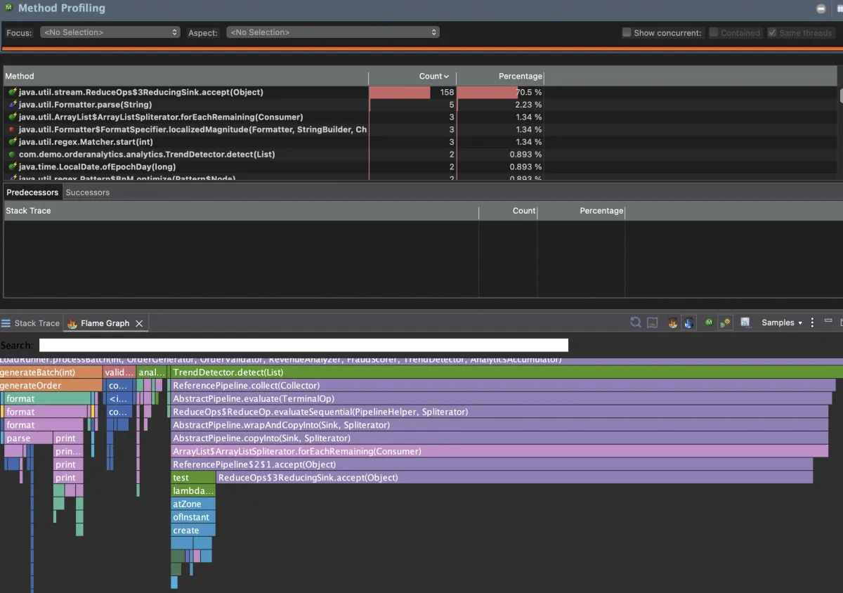
One box is taking up over 70% of the samples. That’s the app spending nearly three quarters of its CPU time in one place.
Notice this maps to java.util.stream.ReduceOps$3ReducingSink.accept(). That’s JDK stream internals. The flame graph shows you what’s hot at the leaf level, which is often a JDK method. To find the problem, you trace up the stack.
Dive in and you’ll see TrendDetector.detect() (my code).
for (Order order : orders) {
    int hour = order.timestamp().atZone(ZoneId.systemDefault()).getHour();

    long countForHour = orders.stream()
        .filter(o -> o.timestamp().atZone(ZoneId.systemDefault()).getHour() == hour)
        .collect(Collectors.counting());

    ordersByHour.put(hour, countForHour);
}
For each order, it streams the entire list to count how many orders share that hour. With 1,000 orders per batch, that’s 1,000 iterations times 1,000 stream elements (a million operations per batch for what should be a single pass). This is the O(n²) stream-inside-loop pattern from Part 1. It was the single largest CPU hotspot, accounting for roughly 70% of all CPU samples in the recording.
While digging into the recording, I also spotted RevenueAnalyzer.analyze() doing string concatenation in a loop, and OrderValidator.validate() calling Pattern.compile() on every invocation, meaning costly regex compilation on every single order. These are immutable, thread-safe objects that should be compiled once and reused, same principle as the recreating reusable objects pattern from Part 1.
Round 1: The Obvious Fixes
Three problems, all visible in the first recording. I fixed them:
1. TrendDetector: O(n²) stream-in-loop → single-pass accumulation
for (Order order : orders) {
    int hour = order.timestamp().atZone(ZoneId.systemDefault()).getHour();
    ordersByHour.merge(hour, 1L, Long::sum);
}
One pass. O(n). Each order increments its hour’s count directly.
2. RevenueAnalyzer: string concatenation → StringBuilder
StringBuilder formattedSummaryBuilder = new StringBuilder();
for (Order order : orders) {
    double revenue = (double) order.quantity() * order.unitPrice();
    formattedSummaryBuilder
        .append("Order ").append(order.orderId())
        .append(" | ").append(order.currency())
        .append(" | Revenue: ").append(String.format("%.2f", revenue))
        .append("\n");
}
Single mutable buffer. No intermediate string copies.
3. OrderValidator: per-call regex compilation → static final patterns
private static final Pattern ORDER_ID_PATTERN = Pattern.compile("ORD-\\d{8}");
private static final Pattern SKU_PATTERN = Pattern.compile("[A-Z]{3}-\\d{4}");

public ValidationResult validate(Order order) {
    // uses ORDER_ID_PATTERN and SKU_PATTERN directly
}
Compiled once at class load and reused on every call.
I re-ran the load test and collected a new recording:
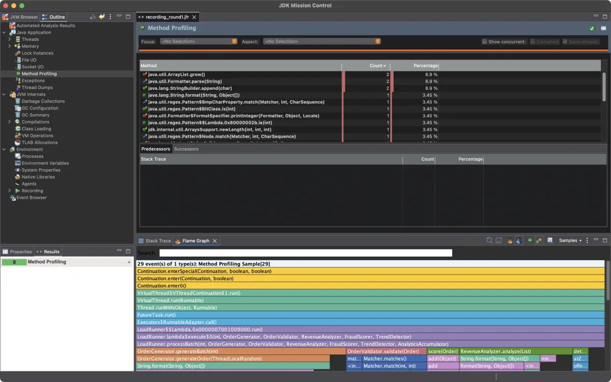
The 70% box is gone. Elapsed time dropped from around 1,000ms to around 400ms. The profile looks completely different.
But look at what’s showing up now. With the TrendDetector hotspot out of the way, the profiler sees things that were previously buried in the noise.
Round 2: What Was Hidden Before
OrderGenerator.generateOrder() is now one of the more visible methods in the profile. It calls String.format() three times per order to build IDs:
String orderId = String.format("ORD-%08d", rng.nextInt(0, 100_000_000));
String customerId = String.format("CUST-%06d", rng.nextInt(0, 1_000_000));
String productSku = SKU_PREFIXES[rng.nextInt(SKU_PREFIXES.length)]
        + "-" + String.format("%04d", rng.nextInt(0, 10_000));
With 100,000 orders, that’s 300,000 String.format() calls. Each one parses the format string, runs the full java.util.Formatter machinery, and allocates intermediate objects. This is the String.format() in hot paths problem from Part 1, different use case (zero-padding IDs instead of building summaries) but same overhead. It was always there. The TrendDetector cost was just louder and was drowning it out.
Fixed it by replacing String.format() with a simple zero-padding helper:
String orderId = "ORD-" + padLeft(rng.nextInt(0, 100_000_000), 8);Along with a handful of other smaller fixes I found while in the code (autoboxing in FraudScorer, string concatenation inside a synchronized method in AnalyticsAccumulator, suboptimal collection choices in ReportGenerator), the elapsed time dropped from around 400ms to around 230ms.
Re-ran and collected a new recording.
The profile is flat. No single dominant hotspot. CPU time is spread across the actual business logic, which is what you want to see. The app is spending time doing work instead of fighting itself.
The Problem the Default Recording Didn’t Show
The flame graph showed me the CPU hotspots. The allocation view showed me the heap pressure. But there’s a third category of performance problem that neither of those surfaces: thread contention.
The default recording ran 100 virtual threads. At that concurrency level, the synchronized method in AnalyticsAccumulator didn’t cause enough lock contention to cross JFR’s reporting threshold. The lock waits were too short to notice.
I got interesting results when I re-ran with higher concurrency, 2,500 virtual threads processing 500,000 orders in batches of 200:
java -XX:StartFlightRecording=filename=contention.jfr,settings=profile \
  -cp target/classes com.demo.orderanalytics.App \
  --orders 500000 --batch-size 200
Now the Contention tab lights up.
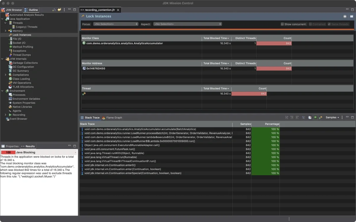
842 monitor contention events. Every single one on AnalyticsAccumulator.accumulate(). Virtual threads queuing up waiting to enter the synchronized method. This is the too-broad synchronization pattern from Part 1, showing up live in the profiler. Median wait time: 15ms. Total aggregate wait time across all threads: over 16 seconds.
This is the thing about contention: it’s load-dependent. At 100 virtual threads it was invisible. At 2,500 it became the bottleneck. If you only profile at low concurrency, you’ll miss it entirely.
There are two ways to attack this. You can replace synchronized with ReentrantLock, which allows more granular lock management and avoids the coarse monitor semantics:
private final ReentrantLock lock = new ReentrantLock();

public void accumulate(BatchAnalytics batchResult) {
    lock.lock();
    try {
        // ... merge results
    } finally {
        lock.unlock();
    }
}
Or you can reduce the work inside the critical section. In this case, replacing string concatenation with StringBuilder means the lock is held for less time on each call, reducing the window where other threads are blocked. In practice, I’d do both.
Results
When I ran this for my DevNexus talk, the numbers from a specific run were:
| Metric | Before | After |
|---|---|---|
| Elapsed time | 1,198ms | 239ms |
| Throughput | 85K orders/sec | 419K orders/sec |
| Peak heap | 1,021MB | 139MB |
| GC pauses | 19 (34ms total) | 4 (6ms total) |
Re-running the same workload for this post, I see similar ratios. Baseline around 1,000ms, optimized around 230ms. The exact numbers shift between runs, but the improvement is consistently 4-5x on elapsed time and over 10x on peak heap.
The seven fixes:
| Fix | Location | Anti-Pattern (Part 1) |
|---|---|---|
| O(n²) stream-in-loop → single-pass | TrendDetector.detect() | Streaming full list per element |
| String concat in loop → StringBuilder | RevenueAnalyzer.analyze() | O(n²) string copying |
| Regex recompilation → static Pattern | OrderValidator.validate() | Recreating reusable objects |
| String.format() → direct string building | OrderGenerator.generateOrder() | Formatter overhead in hot path |
| Autoboxing → primitive arrays | FraudScorer.score() | Wrapper object allocation |
| String concat → StringBuilder | AnalyticsAccumulator.accumulate() | Allocation inside critical section |
| LinkedList/Hashtable → ArrayList/HashMap | ReportGenerator.generate() | Suboptimal collection choices |
Why This Matters at Scale
As I wrote in Part 1, these improvements compound across a fleet. On a single instance, going from 1,000ms to 230ms is a nice win. Across a fleet of instances all handling the same workload, it changes the economics.
It’s hard to convince your boss you should spend two weeks shaving 50ms off a request. Imagine the conversation when you frame it as cost savings. “Let me spend two weeks and we’ll save five figures on our annual infrastructure costs.”
If a 5x throughput improvement means you can handle the same load on fewer instances, or downsize your instance types, run the math on your own fleet. The savings compound fast.
What the Profile Is Actually Telling You
The most useful thing I can pass on: don’t start with the flame graph.
The flame graph shows you hot compute methods. But not every performance problem shows up there. If your bottleneck is excessive allocation, you’ll see it in heap growth and GC frequency before you see it in CPU samples. If your bottleneck is synchronization, you’ll see it in the Contention tab, not the flame graph at all. CPU can look completely normal while threads are stalled waiting on a lock. And as I showed above, contention might not even show up until you profile under realistic production concurrency.
So start with the overview tab. If heap is climbing and GC is running constantly, go to the allocation view first. If CPU is high but heap is flat, go to the flame graph. If CPU is low but response times are slow, go to the Contention tab. Something is blocking.
The other thing worth saying: fix one thing at a time and re-profile. It’s tempting to batch all your changes and just run the benchmarks at the end. The problem is you won’t know what each change actually did. And more importantly, you’ll miss the second-order effects. The String.format() problem in Round 2 only became visible after the Round 1 fixes cleared the noise. Fixing the TrendDetector alone dropped elapsed time from around 1,000ms to around 400ms. But that revealed the String.format() overhead in OrderGenerator, and fixing that dropped it further to around 230ms. If I’d fixed everything at once and just looked at the final numbers, I would have gotten the same result but I wouldn’t have understood why.
One more thing. Look at the fixes in this post. Replacing a stream-in-loop with Map.merge(). Using StringBuilder instead of string concatenation. Hoisting Pattern.compile() to a static field. Most of these made the code both faster and cleaner. If you find yourself in a position where optimizing is making the code harder to read or maintain, that’s worth pausing on. Focus on the changes that will have impact when running at scale, and keep the code something your team can live with.
Doing This on Your Own App
You need two things: a JFR recording from a load test or a production traffic window, and JMC to open it.
# Start recording at launch with comprehensive event capture
java -XX:StartFlightRecording=filename=myapp.jfr,settings=profile -jar myapp.jar

# Or attach to a running process
jcmd <pid> JFR.start duration=120s filename=myapp.jfr settings=profile
JFR is included in OpenJDK since Java 11 (and backported to OpenJDK 8u262). Overhead is under 1% in most configurations. You can run it in production. Use settings=profile to get the full picture: CPU sampling, allocation tracking, GC events, and thread contention.
Once you have the file:
- Open it in JMC
- Start with the overview tab to understand the shape of the problem
- Heap climbing and GC pressure → go to the Allocation view
- High CPU → go to Method Profiling and the flame graph
- Slow response times with normal CPU → go to the Contention tab under Threads
- Fix the loudest problem first, re-profile, then repeat
And if contention is a concern, profile under realistic concurrency. A lock that’s invisible at 10 threads can become the bottleneck at 1,000.
That last point is the whole workflow. It’s not a one-shot process. Each round of fixes changes what’s visible in the next recording.
The full source code for the demo app is on GitHub. The main branch has the unoptimized code with all the anti-patterns intact. The performance-optimized branch has the fixes. You can diff the two to see exactly what changed.
In Part 3 we’ll look at how to automate this loop entirely. The JFR data has enough signal to drive the fixes programmatically, and there are tools that can read it, rank the anti-patterns by hot path weight, write the code changes, run your tests, and hand you a diff. We’ll walk through exactly what that looks like.
Something you’re seeing in your own JFR recording that doesn’t make sense? I’m on LinkedIn.
Part 3 coming soon.